Geometry: Transformation of the Plane II
The following are images of transformations in the plane.
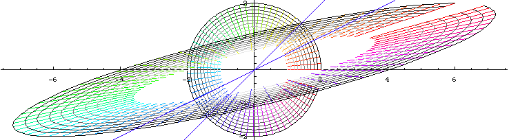
{{3,-2},{1,0}}. The matrix has two independent eigenvectors {1,1} and {2,1}, indicated by blue lines. Their significance is that points on those lines will remain on those lines.
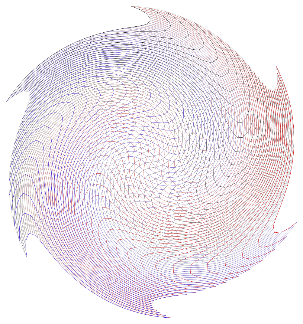
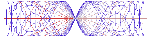
Clear[n]; n = N[Pi/3];
Transform2DGraphicsPlot[TriangularGrid[Pi, 49],
   Function[{x,
   y}, ({{Cos[#1*n], -Sin[#1*n]}, {Sin[#1*n], Cos[#1*n]}} & )[
    Norm[{x, y}]] . {x, y}], ResolutionLength -> 0.2,
   AspectRatio -> Automatic]

Sin[Norm[v]] * 0.4 * Normalize[v] + v applied to a wallpaper design.
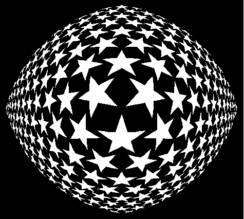
Function[{#1,#2}/(Sqrt[#1^2 +#2^2] + 5)] applied to a wallpaper design of stars. This function is often called fish-eye lens.
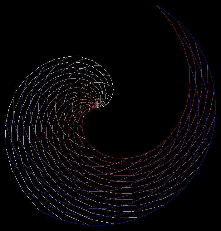
Function[{#2, Cos[#1*#2]}] applied to a polar grid.
Notation Used
These graphics are generated by my Mathematica packages Transform2DPlot.m and PlaneTiling.m. You can get them at Wolfram: Transform2DPlot Package 📦 and Wolfram: Plane Tiling Package 📦 .