Geometry: Transformation of the Plane
What follows are images of Transformation of the Plane. The original image is a square grid or polar grid. The transformed image is shown, under a function ƒ. For most images, the coloring is done by a function that measures the change of distance from the point to the image of the point under ƒ.
These graphics are generated with the Mathematica package Transform2DPlot.m. You can get it at Mathematica Package: Geometric Transformation on the Plane .
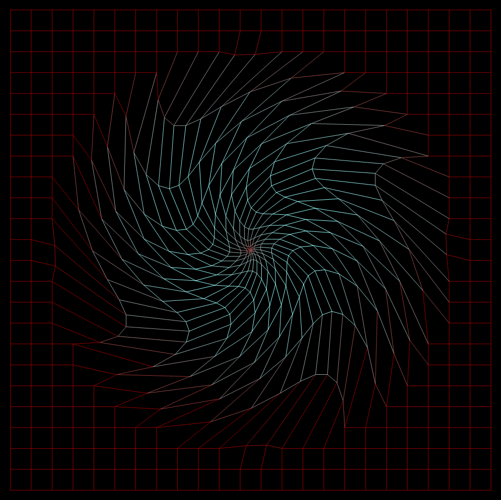
pastelSpin

Clear[n];
n = N[Pi/3];
Transform2DPlot[({{Cos[#1*n], -Sin[#1*n]}, {Sin[#1*n], Cos[#1*n]}} & )[
       Norm[{x, y}]] . {x, y}, {x, -2*Pi, 2*Pi}, {y, -2*Pi, 2*Pi},
   PlotRange -> {{-1, 1}, {-1, 1}}*3.1, ColorFunction ->
     (Hue[RandomReal[], Sqrt[#1], 0.8] & ), PlotPoints -> 47,
 Axes -> False]
blackhole
Clear[f, n]
n = N[2];
f[x_, y_] := If[N[Sqrt[x^2 + y^2]] < 1,
     ({{Cos[(1 - #1)*n], -Sin[(1 - #1)*n]}, {Sin[(1 - #1)*n],
                  Cos[(1 - #1)*n]}} & )[x^2 + y^2] . {x, y}*(x^2 +
     y^2), {x, y}]
Transform2DPlot[f[x, y], {x, -1.2, 1.2}, {y, -1.2, 1.2},
 Axes -> False,
   Background -> GrayLevel[0],
 ColorFunction -> RandomRGBColorFunctionGenerator[
       ], PlotPoints -> {24, 24}]
fishnet
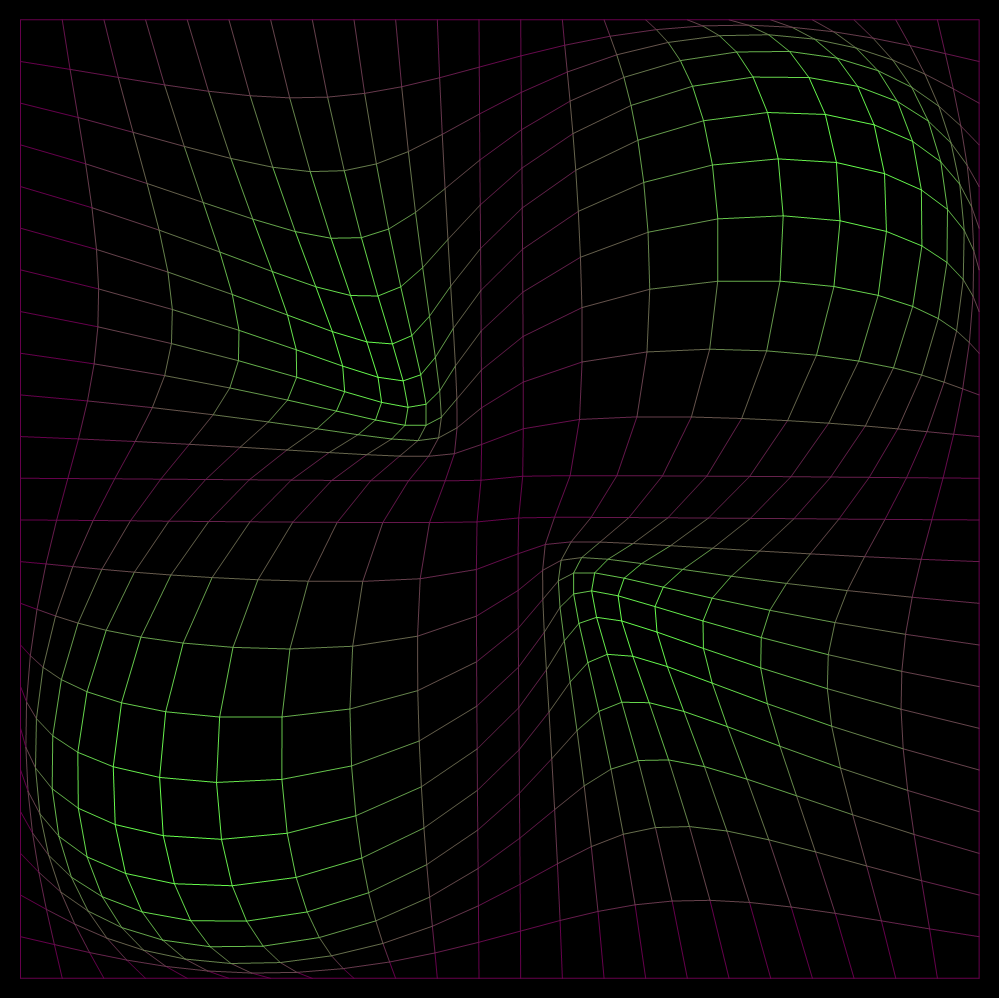
Transform2DPlot[(Sin[x]*Sin[y])*Normalize[{x, y}] + {x, y}, {x, -Pi, Pi},
  {y, -Pi, Pi}, PlotPoints -> 24*{1, 1}, ColorFunction ->
   (RGBColor[0.4, #1, 0.3] & ), Background -> GrayLevel[0], Axes -> False]
sinewave
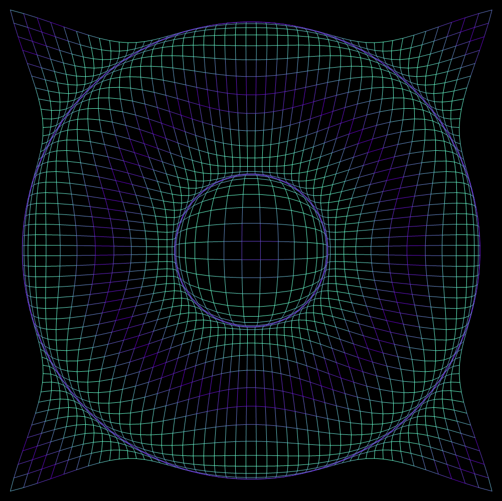
Transform2DPlot[Sin[Sqrt[x^2 + y^2]]*Normalize[{x, y}] + {x, y},
   {x, -3*Pi, 3*Pi}, {y, -3*Pi, 3*Pi}, PlotPoints -> {1, 1}*50,
   ColorFunction -> (RGBColor[0.4, #1, 0.8] & ),
 Background -> GrayLevel[0],
   Axes -> False]
burned hole
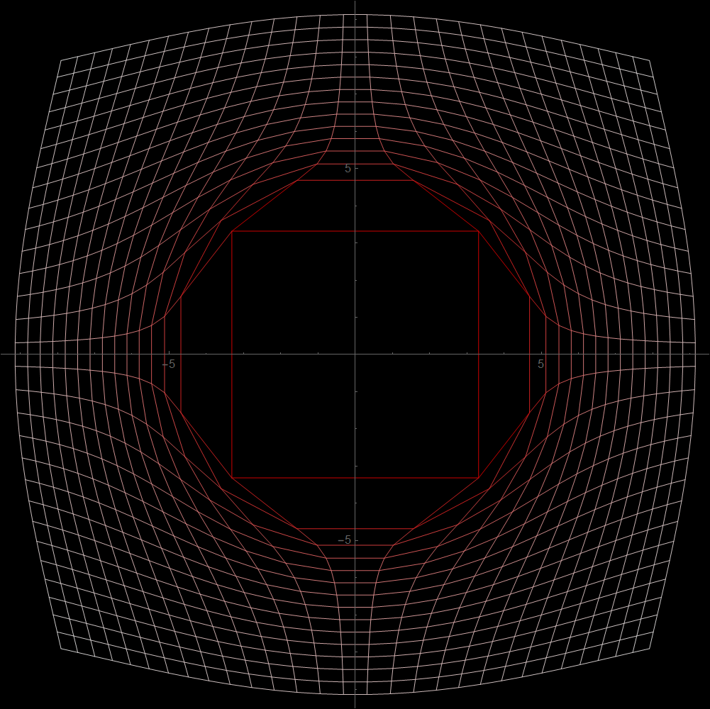
Transform2DPlot[Normalize[{#1, #2}]*(1/(Norm[{#1, #2}] + 2) + 4) +
       {#1, #2} & , {-1, 1}*5, {-1, 1}*5, PlotPoints -> {1, 1}*30,
 Axes -> True,
   Background -> GrayLevel[0]]
magGlass
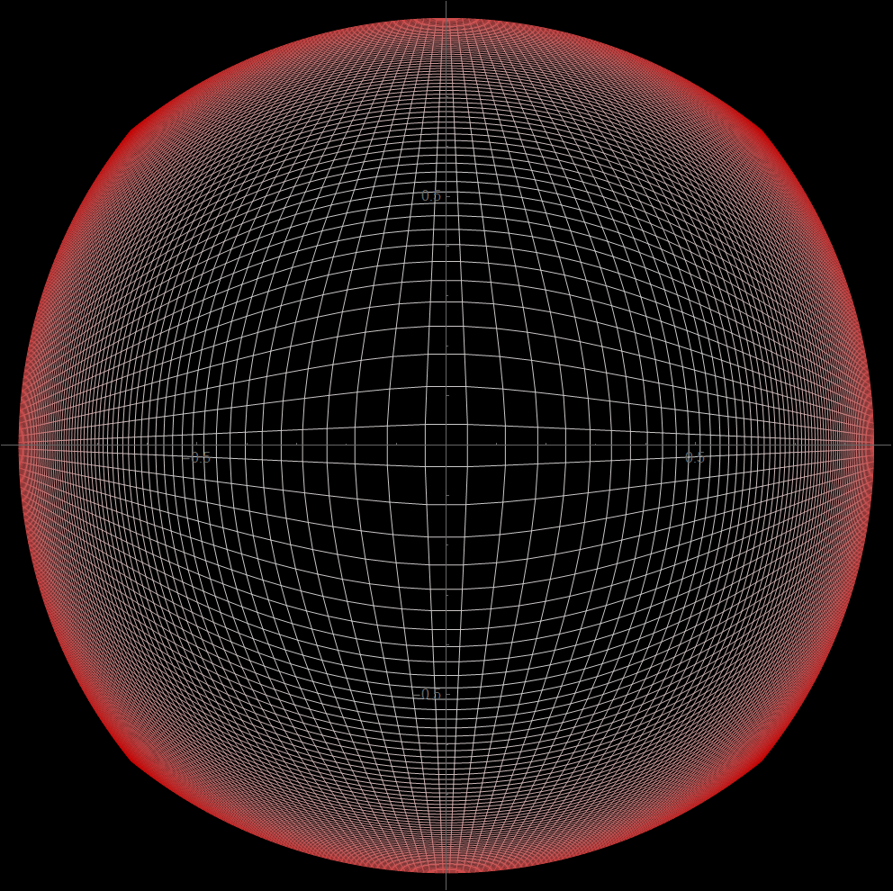
Transform2DPlot[{#1, #2}/(Norm[{#1, #2}] + 1/2) & , {-1, 1}*3, {-1, 1}*3,
   PlotPoints -> {1, 1}*134, Background -> GrayLevel[0]]
complexInv
Transform2DPlot[1/(x + y*I), {x, -2, 2},
  {y, -2, 2}, PlotPoints -> {1, 1}*50,
  ColorFunction -> (RGBColor[0.7,
     -(#1 - 1)^4 + 1, 0.1] & ),
  PlotRange -> {{-1, 1}, {-1, 1}}*3.6,
  Background -> GrayLevel[0], Axes -> False]
log

Transform2DPlot[{Log[x + 0.001], Log[y + 0.001]}, {x, 0, 3}, {y, 0,
  3}, ColorFunction -> Hue]
tan cross

Transform2DPlot[Tan[{x, y}], {x, -1.5, 1.5}, {y, -1.5, 1.5},
 PlotPoints -> {1, 1} 24, ColorFunction -> Hue, Axes -> False,
 Background -> GrayLevel[0]]
fan

GraphicsGrid@
 Function[{x}, Partition[x, 3]]@
  Table[Transform2DPlot[
    Sin[Norm[{x, y}]] Normalize[{x, y}], {x, -i, i}, {y, -i, i},
    Axes -> True], {i, Pi/2, Pi, Pi/(2 5)}]
explosion

Transform2DPlot[
 Sin[x y] {x, y}, {x, -2 Pi, 2 Pi}, {y, -2 Pi, 2 Pi},
 Background -> GrayLevel[0], Axes -> False]
Amethyst

GraphicsGrid @
Function[{x}, Partition[x,3]] @
Table[Transform2DPlot[
  Sin[Norm[{#1, #2}]] {#1, #2} &, {-1, 1} i, {-1, 1} i,
  ColorFunction -> (Hue[.9, #1, .8] &), Background -> GrayLevel[0],
  Axes -> False, PlotRange -> {{-1, 1}, {-1, 1}} 3], {i, Pi, 2 Pi, Pi/5}]
roller coster

Transform2DPlot[{y, Sin[y x]}, {x, 0, Pi}, {y, 0, 2 Pi},
 PlotPoints -> {1, 1} 24, ColorFunction -> Hue, Axes -> True,
 Background -> GrayLevel[0], Ticks -> {Range[0], Range[-5, 5, 1]}]
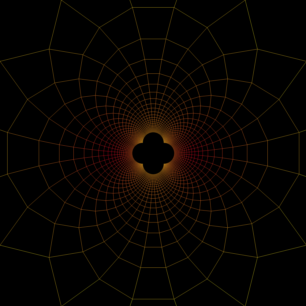
tit

Transform2DGraphicsPlot[
 PolarGrid[{0.1, 2}, {0, 2 3.14156}, {Hue[0.7, #1, 0.7] &,
   Hue[0, 1 - #1, 0.7] &}],
 Function[{x, y}, 1/(Norm[{x, y}] + 1) + {x, y}],
 ResolutionLength -> 0.1, AspectRatio -> Automatic]
Mathematica Notation
What is Transformation
A transformation in the plane is a function that maps a point in the plane to another point in the plane, for all points in the plane (or a region). Put it another way, a function f that takes coordinate {a,b} and out put a point {c,d}. A transformation is also called a mapping or function. It is usually called transformation in geometry context.
When doing a transformation in the plane, we start with a image in the plane.
For example, lines, circles, curves, or any figure.
The starting image is usually called pre-image, and the figure after transformation is called image.
For example, suppose we start with a circle of radius 1 centered on the origin.
Suppose our function is f[{x,y}]:={x+1,y+1}.
Then, after the transformation, the image would be a circle of radius 1 centered on {1,1}.
In the above illustrations, the pre-image is a grid.
One-to-one Mapping
There are many classification of transformations. First of all, we can classify a transformation by asking whether if 2 or more points are mapped into the same point. If not, then it is called a one-to-one mapping.
A easy way to think of one-to-one, is that there are no overlaps. A non-one-to-one transformation will have overlapping points.
Most transformations studied in geometry are the one-to-one type. A reflection (mirroring), a rotation, a scaling (dilation/contraction), or a translation (shifting, pan) are all one-to-one transformations.
Continuity
We can also classify transformations into continuous and discontinuous. It asks whether neighbors points remain neighbors. Suppose you cut out two circles in a paper, swap their locations and tape them back. Obviously, the points on the boundary of the circles now has new neighbors, after the transformation. Such is a discontinuous transformation because it cuts continuity.
Rotation, translation, reflection, are all continuous transformations. Most transformations studied in geometry are continuous transformations.
Distance-preserving
Transformations are classified by many other ways. We may ask whether distance is preserved. Reflection, rotation, translation are this type. Scaling (dilation/contraction) or shearing do no preserve distance. Distance-preserving transformations are called isometry. It is also called rigid motions.
Sense-preserving
Another distinction is whether the orientation (also called sense) is preserved. Suppose you have the letter P in your plane. After a reflection, P will be reversed. Thus reflection is a sense-reversing transformation. On the other hand, you can never reverse P by a rotation, scaling, or a translation.
Linear Transformation
A important class of transformation, is transformations such that preserve a line thru the origin. That is, if you have a line passing the origin, then, after transformation, is image of this line still a line passing the origin? If so, it is called linear transformations .
Rotation around the origin, dilation around the origin, reflection around the origin, and shearing, are all linear transformations.
Affine Transformation
A more broader class of transformation is called affine transformation (aka affinity). Affine transformation includes all linear transformation plus any combination of them with translation.
Viewed in another way, it asks if parallel lines are preserved. If two parallel lines are still parallel lines after the mapping, then this mapping is a affine transformation.
Conformal Transformations
Another important class of transformation is called conformal maps or conformal transformations. It asks whether angles are preserved. Suppose you have two lines in your plane that forms a angle α. Now after your transform, do they still form angle α?
Such transforms are studied in a branch of math called complex analysis. A particular interesting conformal map is called inversion. Imagine the plane as huge piece of paper. Now punch a hole in the center of the paper, poke in both of your thumbs inside, with the rest of your fingers grabbing the edges of the paper. Now flip the paper inside out, so that the edge in the hole are on the outside, while the paper's edge becomes the boundary of the hole. (this is not possible to do in real life, but just imagine) Now seal up the hole, and done, that's inversion. Points in the center are mapped to far away (infinity) and points far away are mapped to the center. You essentially turned a plane inside out. Amazingly, this process preserve angles. (For detail, see: Inversion and Nested Inversion of Circles.)
Projective Transformation
Suppose you take a crayon and draw figures on a glass pane. Then take this glass pane outside so the sun cast shadows on the ground. Now, each point in your figure has a corresponding point on the ground. This transformation is called projective transformations (aka projectivity.).
The property projectivity preserves is incidence and cross ratio. Incidence means whene 2 curves cross. In a projectivity, if 2 curves cross at n points, then after the transformation they will still meet at n points. Cross ratio means the ratio of 2 segments defined by 4 points on a line. In projectivity, this ratio is preserved.
For more about projective transform, see:
Topological Transformations
Another class of transformations, is called Homeomorphism. This class are basically transformations that are continuous, and is studied in a branch of math called Topology. Basically, you can now think of the plane as a piece of rubber of infinite extent. You can pinch, stretch, and distort it any way you like, as long as you don't cut or tear. You can draw a smiley on the rubber and make it grin from east to west. In topological transforms, shapes are not distinguished. Circles and triangles are considered the same, but nevertheless certain properties of figures remain. For example, a loop will never become a line. Here's one theorem from topology, Jordan curve theorem: You can never connect a point inside a loop to a point outside without crossing the loop.
Xah Talk Show, Transformation of the Plane
