Geometric Inversion
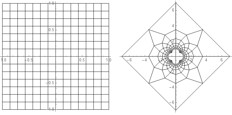
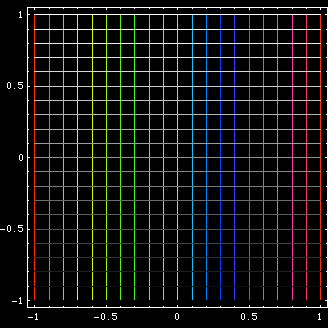
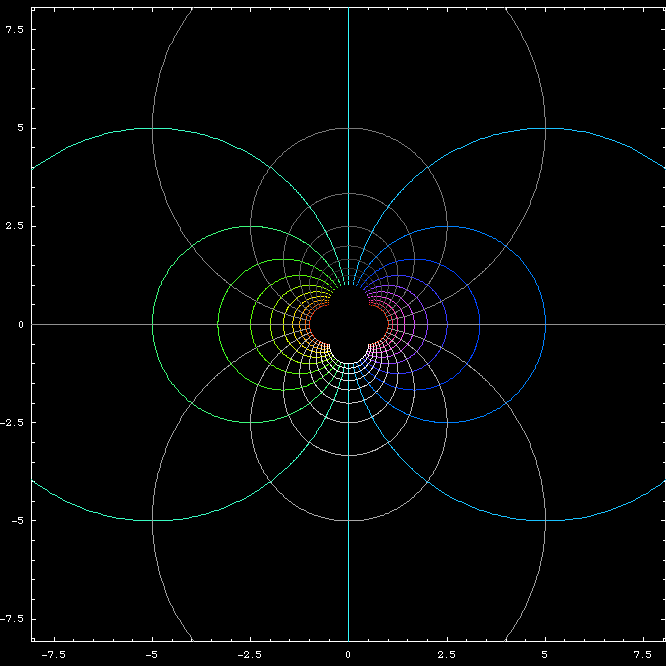
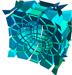
geoInv = Function[x, ((With[{x930 = x . x}, If[x930 < 0.00000001, x, x/x930]]) )];
cArray = CoordinateBoundsArray[{{-1, 1}, {-1, 1}}, Into[14]];
vLines = Function[x, (BlockMap[Line, x, 2, 1] )] /@ cArray;
hLines = Function[x, (BlockMap[Line, x, 2, 1] )] /@ Transpose@cArray;

gp1 = {hLines, vLines};
gp2 = gp1 /. Line[x_] :> Line[geoInv /@ x];

gr1 = Graphics[gp1, Axes -> True]
gr2 = Graphics[gp2, Axes -> True]

GraphicsGrid[{{gr1, gr2}}]
History
Geometrical inversion seems to be due to Jakob Steiner (“the greatest geometer since Apollonius”) who indicated a knowledge of the subject in 1824. He was closely followed by Adolphe Quetelet (1825) who gave some examples. Apparently independently discovered by Giusto Bellavitis 〔https://mathshistory.st-andrews.ac.uk/Biographies/Bellavitis/〕 in 1836, by Stubbs and Ingram in 1842-3, and by Lord Kelvin in 1845. The latter employed the idea with conspicuous success in his electrical researches. (Robert Yates: Curves and Their Properties.)
Description
Geometric Inversion
Geometric Inversion is a transformation. Let P be a given point. Let c be a circle centered on O and radius r. The inverse of P with respect to c is a point Q on the line[O,P] such that distance[O,P] * distance[O,Q] == r^2.
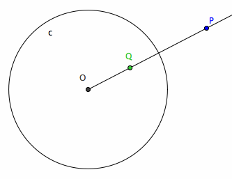
From this definition, few properties can be seen easily:
- Q is a inverse of P if and only if P is a inverse of Q.
- Points inside the circle are mapped to the outside and vice versa.
- Points on the circle are fixed points (i.e. the inversion of any point on the inversion circle is itself).
The center of the inversion circle is called the pole.
Inversion Of A Curve
The inversion of a curve is the inversion of all points on the curve.
- If curve A is the inverse of curve B, then curve B is also the inverse of curve A with respect to the same circle.
- Curves that inverts into themselves are called anallagmatic curves. Circles, lines, and Cassinian ovals are anallagmatic curves.
- Asymptotes to a curve C invert into a curve that is tangent C's inverse.
- The radius of inversion circle effects the scale of the inversion curve, but not its shape.
Formula
Point in Rectangular Coordinate
The inversion of a point {x,y} with respect to a circle centered at {a,b} and radius r is:
Clear[ geoInversion ]
geoInversion[{x_,y_}, {a_,b_}, r_] := {x-a,y-b}*r^2/((x-a)^2+(y-b)^2) + {a,b}
when the inversion circle is centered at origin with radius 1, we have:
geoInversion[{x,y}, {0,0}, 1] === {x, y}/(x^2 + y^2)
Geometric Inversion Formula Derivation
The derivation can be easily done by thinking in vectors.
Suppose the inversion circle has radius r at origin.
Suppose we have a vector P with coordinates
{x,y}
.
We want to find a vector Q such that
length[P]*length[Q]==r^2
and Q have the same direction as P.
Now, the length of P is
Sqrt[x^2+y^2]
.
We have
length[Q]==r^2/Sqrt[x^2+y^2]
.
The vector Q is a vector in the direction of P with length
r^2/Sqrt[x^2+y^2]
.
We multiply the unit vector in the direction of P with the desired length:
(P/length[P])*(r^2/Sqrt[x^2+y^2])
, which simplifies to
{x,y}*r^2/(x^2+y^2)
This is the formula for inversion of a point {x,y} with respect to a circle centered on origin with radius r.
Now, if the pole O is not at the origin, we can derive the formula by first translating O and P so that O is at the origin, then do the inversion, then translate the inverted point in reverse direction.
In formulas, suppose O is {a,b}, the coordinate of P' is then {x-a,y-b}
and O' is {0,0}.
Applying the inversion formula
{x,y}*r^2/(x^2+y^2)
, we have
{x-a,y-b}*r^2/((x-a)^2+(y-b)^2)
.
Translate it back, we have:
{x-a,y-b}*r^2/((x-a)^2+(y-b)^2) + {a,b}
.
Polar Coordinate
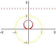
Give a curve with polar formula r==f[θ], its inverse curve with respect to a circle centered on the pole with radius k is
r==k^2/f[θ]
.
Give a curve with parametric formula in polar coordinate:
{f[θ],θ}
, its inverse curve with respect to a circle centered on the pole with radius k is
{k^2/f[θ],θ}
.
Properties
Inversion of Circle
The inversion of a circle or line is a circle or line. Let O denote the center of inversion. We have:
| Curve A | Curve B | |
|---|---|---|
| (A) | line through O | line through O |
| (B) | line not through O | circle through O |
| (C) | circle through O | line not through O |
| (D) | circle not through O | circle not through O |
- Proof: Statement (A) is trivial.
- To prove (B), let A be a point on the line L so that OA and L are perpendicular.
- Let P be any point on L other than A.
- Let A' and P' be the inverse of A and P.
- By the definition of inversion, we have OA'*OA == OP'*OP == r^2.
- By algebra we have OA'/OP' == OP/OA.
- This means triangle[O,P',A'] and triangle[O,A,P] are similar because the ratio of their sides are equal, therefore angle OP'A' is a right angle.
- From the Converse of Thales's Theorem , it follows that P' lies on a circle with diameter OA'.
- This ends the proof of statement (B).
- Proof of statement (C) follows automatically because inversion of points are mutual.
- Proof of (D): Let the intersection of the circle and a line thourgh O be P and Q.
- Let P', Q' be their images.
- Let M be the center of the given circle.
- We have OP*OP' == OQ*OQ' == r^2 by the definition of inverse.
- Also, OP*OQ == OM^2-r^2 from a elementary theorem on circle.
- Divide the first equation by the second we get OP'/OQ == OQ'/OP == r^2/(OM^2-r^2), which is a constant.
- Through Q' we draw a line parallel to PM.
- Let the intersection of the line and OM be N.
- We have now triangles OQ'N and OPM.
- Since these triangles has two sides parallel, they must be similar, thus OQ'/OP == Q'N/PM == NO/MO.
- Solve for NO we get NO == MO*OQ'/OP == MO*r^2/(OM^2-r^2).
- Solve for Q'N we have Q'N == PM*OQ'/OP == r*r^2/(OM^2-r^2).
- Both of which is a constant.
- This means for any point P on the circle, Q'N and NO are constant.
- Similarly, for any point Q on the circle, P'N and NO are constant.
- Thus P' and Q' must be points on the same circle.
- End of proof.
From the formula of a inversion of a point, and the theorem that circle invert to circles, we can easily derive the formula of a Circle[{c1, c2}, s] inverted wrt Circle[{o1, o2}, r], is:
Circle[({c1, c2} - {o1, o2})/oc*(oc r^2/(oc^2 - s^2)) + {o1, o2},
 Abs[r^2 s/(oc^2 - s^2)]]
where oc is the distance from {c1,c2} to {o1,o2}
Invariance of Angles
Angles are preserved under inversion with reversed sense. That is, if two curves intersect with angle α, their inverse will also intersect with angle α but in a reversed direction of sweeping.
GeoGebra: Inversion Angle Invariance
Peaucellier Linkage
Peaucellier Linkage is a mechanical contrivance for tracing the inverse of a curve. It is named after Charles-Nicolas Peaucellier (1832 to 1913) who discovered it in 1864. The significance of this simple linkage is that it solved the problem of converting a circular motion to a linear motion by a linkage that was believed to be impossible at the time.
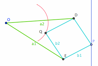
The linkage consists of six arms of fixed length (green and light blue lines in figure above), and five joints (point O, P, Q, E, D). To generate a inverse of a given curve (For example, a line in blue), fix point O in the plane and move P along the curve. The trace of Q will be the inverse of C with respect to O and radius Sqrt[a^2-b^2], where a and b are the length of the arms. To convert circular motion to linear motion, we simply need to restrain the motion of Q on a fixed circle passing O.
- Proof:
- We need to show such device with any degree of opening will have OP * OQ == r^2 for a constant r.
- Let x = ED/2, thus x represents the variable opening of the device.
- We have OP == Sqrt[a^2-x^2] + Sqrt[b^2-x^2], OQ == Sqrt[a^2-x^2] - Sqrt[b^2-x^2].
- Then OP * OQ == a^2-b^2, after simplification.
- End of Proof.
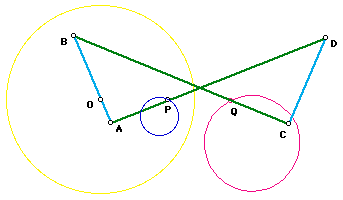
Hart's Linkage
Hart's Linkage is another mechanical contrivance for tracing the inverse of a curve. The linkage consists of four arms of fixed length (green and light blue lines in figure below), four joints (point A, B, C, D), and three positions (O, P, Q) fixed on the arms. The two lengths (AB==CD, BC==AD) of the four arms are arbitrary. The fixed positions O, P, Q on the arms are also arbitrary with the condition that O, P, Q must be collinear and parallel to AC. To trace a inverse of a given curve (For example, a circle in blue), fix point O in the plane and move P along the curve. The trace of Q (pink) will be the inverse with respect to O.
- Proof:
- We want to show that OP * OQ == r^2 for some constant r, no matter what design or position of Hart's linkage.
- We note that points A, B are symmetric to C, D because AB==CD, BC==AD, thus AC, BD, OP are all parallel.
- Triangle AOP and ABD are simular, thus OP/BD == AO/AB.
- Similarly, triangle BOQ and BAC implies OQ/AC == BO/BA.
- Combine the last two equations we get OP*OQ == (AO)*(BO)*(BD)*(AC)/(AB)^2.
- Now we just need to show the quantity (BD)*(AC) is a constant.
- Let E, F be the parallel projection of point A, C on the line B, D.
- So we have right triangles AEB and CFD.
- Now BD*AC == BD*EF == (ED+EB)*(ED-EB) == ED^2 - EB^2.
- We know that ED^2 + AE^2 == AD^2 and EB^2 + AE^2 == AB^2.
- Combine the last three equations to get ED^2 - EB^2 == AD^2 - AB^2.
- This quantity is a constant regardless the positions of the linkage.
- End of Proof.
We have derived the radius of inversion with Hart's linkage is r == Sqrt[ (AO)*(BO)*/(AB)^2*(AD^2 - AB^2)].
Note that if we constrain point P of Peaucellier or Hart's linkage to move around a circle that passes point O, we have a mechanism that converts circular motion to linear motion.
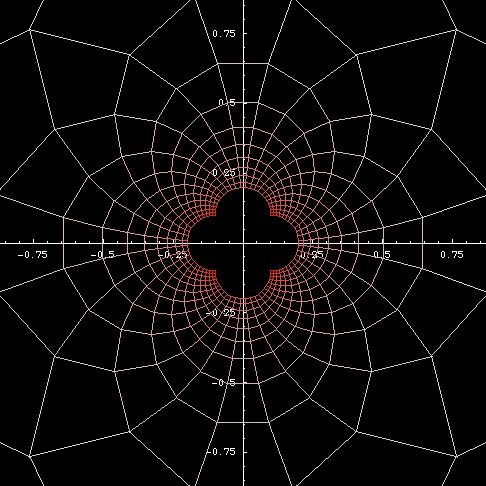
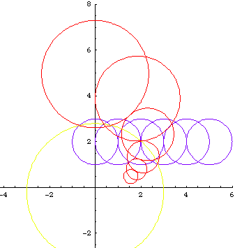
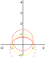
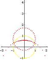
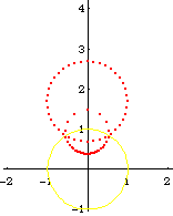
Circle Inversion Gallery
Curve relations by inversion
| Curve | Center of Inversion | Curve |
|---|---|---|
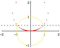
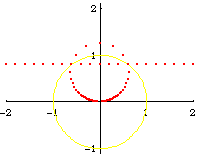
| line | not on line; on circumference | circle |
| circle | not on circumference | circle |
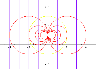
| conics | focus; pole | limacon of Pascal |
| ellipse, hyperbola | center | Oval?, lemniscate of Gerono |
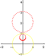
| parabola | focus; cusp | cardioid |
| parabola | vertex; cusp | cissoid of Diocles |
| rectangular hyperbola | center | lemniscate of Bernoulli |
| rectangular hyperbola | vertex; node | right strophoid |
| hyperbola, e:=2/Sqrt[3] | vertex; node | trisectrix of Maclaurin |
| trisectrix of Maclaurin | focus; -- | Tschirnhausen's cubic |
| right strophoid | pole | right strophoid |
| equiangular spiral | pole | equiangular spiral |
| Archimedean spiral | pole | Archimedean spiral |
| lituus | pole | parabolic spiral |
| sinusoidal spiral | pole | sinusoidal spiral |
| epispiral | pole | rose |
| cochleoid | pole; -- | quadratrix of Hippias |
Misc
 Geometric Inversion, WolframLang Code