Xah Talk Show 2025-03-26 Ep635 Wolfram language, graphics for beginner, draw pedal curve

xah talk show 2025-03-26 14509

graphics basics

(* graphics primitives *)

Circle[ {0,0}, 1 ]
Line[ {{0,0}, {0,1}} ]
Polygon[ {{0,0}, {0,1}, {2,3}} ]

(* HHHH------------------------------ *)

(* to show the graphics primitives,
put them inside
 Graphics[]  *)

Graphics[
{
Circle[ {0,0}, 1 ],
Line[ {{0,0}, {2,1}} ],
Polygon[ {{0,0}, {0,1}, {2,3}} ]
},
Axes -> True
]

(* HHHH------------------------------ *)

(* what about color.
color, thickness, are call graphics directives.
 *)

Graphics[
{
{Red, Circle[ {0,0}, 1 ]},
{Blue, Thickness[ 0.1 ], Line[ {{0,0}, {2,1}} ]},
Polygon[ {{0,0}, {0,1}, {2,3}} ]
},
Axes -> True
]
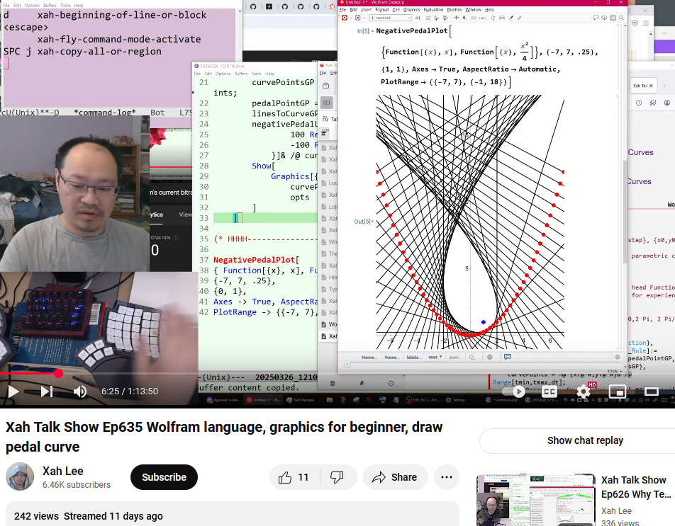
xah talk show 2025-03-26 Wolfram language graphics 1e2f0

graphics program the negative pedal

xah talk show 2025-03-26 Wolfram language graphics 20945
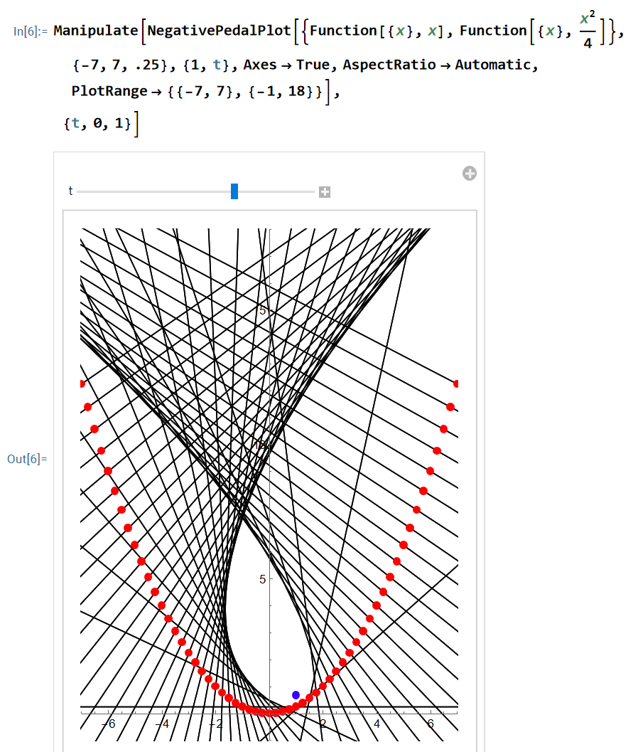
(*
give a curve, parabola, by the formula
{x, x^2}

given a point O, lets say {1,1},
this is called the pedal point.

now, we want to draw a line L,
passing a point P on parabola,
and is perpendicular to the line OP.

and we want to do this for many points P on the curve.
 *)

(* draw points on parabola *)
parabolaPoints = Table[{x, x^2} , {x, -1, 1, 0.1}]
dots = Map[ Point , parabolaPoints]
Graphics[ { Red , dots}, Axes -> True ]
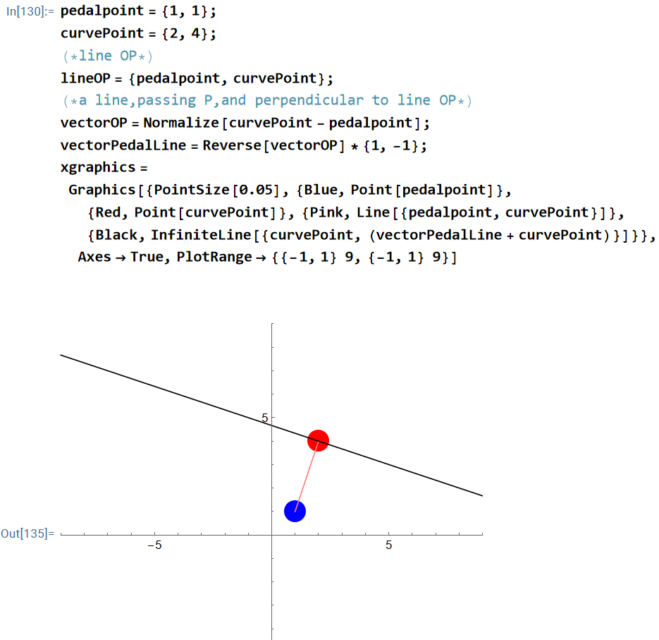
(* HHHH------------------------------ *)

(* draw a line L, that is perpendicular to line OP *)

pedalpoint = {1,1};
curvePoint = {2,4};
(* line OP *)
lineOP = { pedalpoint, curvePoint};
(* a line, passing P, and perpendicular to line OP *)
vectorOP = Normalize[ curvePoint - pedalpoint ];
vectorPedalLine = Reverse[ vectorOP ] * {1,-1};
xgraphics = Graphics[
{
PointSize[ 0.05 ],
{ Blue,  Point[ pedalpoint ]},
{ Red, Point[ curvePoint ]},
{ Pink, Line[ { pedalpoint , curvePoint} ]},
{ Black, InfiniteLine[ {curvePoint, (vectorPedalLine + curvePoint) } ]}
},
Axes -> True,
PlotRange -> {{-1,1} 9, {-1,1} 9}
]
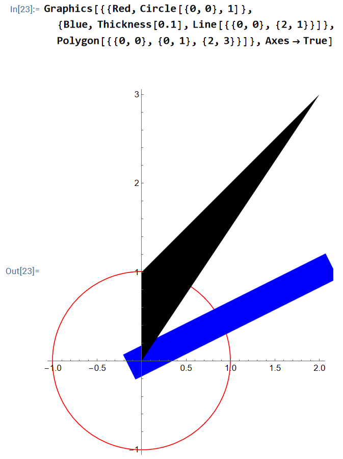
(* to find a vector that is perpendicular to vector {a,b},
is {b, -a}
 *)

Clear[ aa, bb ]
aa = 2;
bb = 3;
vec1 = {aa,bb}
vec2 = {bb, -aa}
Graphics[ {
{ Red , Line[ {{0,0} , vec1} ]},
{ Blue , Line[ {{0,0} , vec2} ]}
}, Axes -> True
 ]

a negative pedal of parabola

xah talk show 2025-03-26 neg pedal parabola
Clear[NegativePedalPlot]

NegativePedalPlot::usage =
"NegativePedalPlot[{xf,yf}, {min,max,step}, {x0,y0}]

draws the negative pedal lines of the parametric curve {xf,yf} at points Range[min,max,step].

xf and yf must be pure functions with head Function.

Example:
NegativePedalPlot[{Cos@#&, Sin@#&}, {0,2 Pi, 2 Pi/30},{.8,0}]";

NegativePedalPlot[{xf_Function,yf_Function},
	{tmin_,tmax_, dt_}, {a_,b_}, opts___Rule]:=
	Module[{curvePoints, curvePointsGP,pedalPointGP,
		linesToCurveGP, negativePedalLinesGP},
		curvePoints = N@ {xf@ #,yf@ #}& /@ Range[tmin,tmax,dt];
		curvePointsGP = {Hue[0],PointSize[.02], Point[#]}& /@ curvePoints;
		pedalPointGP = {Hue[.7], PointSize[.02], Point[{a,b}]};
		linesToCurveGP = N@ Line[{{a,b},#}]& /@ curvePoints;
		negativePedalLinesGP = Line[{
				100 Reverse[Normalize[N[#-{a,b}]]{1,-1}] +#,
				-100 Reverse[Normalize[N[#-{a,b}]]{1,-1}] +#
			}]& /@ curvePoints;
		Show[
			Graphics[{negativePedalLinesGP,
				curvePointsGP, pedalPointGP}],
				opts
		]
	]

(* HHHH------------------------------ *)

NegativePedalPlot[
{ Function[{x}, x], Function[{x}, x^2/4 ] },
{-7, 7, .25},
{0, 1},
Axes -> True, AspectRatio -> Automatic,
PlotRange -> {{-7, 7}, {-1, 18}}]