Mathematica Version 3 to Version 7 Conversion Notes
This page is misc personal notes of learning new features of Mathematica since version 3 in 1996.
HiddenSurface
As of Version 6.0,
HiddenSurface->False
has been superseded by the setting
PlotStyle->FaceForm[]
GraphicsArray → GraphicsRow, GraphicsGrid
GraphicsArray
is replaced by GraphicsRow and GraphicsGrid
ImplicitPlot → ContourPlot
<< Graphics`ImplicitPlot`; is obsolete. Use ContourPlot instead.
<< Graphics`ImplicitPlot`;
ImplicitPlot[{(x^2 + y^2)^2 == x^2 - y^2, (x^2 + y^2)^2 == 2 x y},
 {x, -2, 2},
 PlotStyle -> {GrayLevel[0], Dashing[{.03}]}]
ContourPlot[{(x^2 + y^2)^2 == x^2 - y^2, (x^2 + y^2)^2 == 2 x y},
 {x, -1, 1}, {y, -1, 1},
 ContourStyle -> {GrayLevel[0], Dashing[{.03}]}]
FilterOptions → FilterRules
Random → RandomReal, RandomInteger
v6.0, Random has been superseded by the functions RandomReal and RandomInteger.
v6.0, StyleForm has been superseded by Style.
default input, now StandardForm instead of InputForm
By default the input cell now uses StandardForm instead of InputForm. (if i recall correctly)
Order of symbols in $Context
Order of symbols in$Context seems to have changed.
That is, when loading a package, the exported symbols now override your global ones (goes first in $Context).
Before, when you call a function in a package such as ParaPlot, but you forgot to load the package.
M gives a error.
Then, you load the package, but that won't work, because ParaPlot is in the Global`
context and that has precedence than the one in Graph`ParaPlot.
This used to be a big problem. Now, this seems fixed. Haven't thought about logical consequences yet.
Graphics Display Behavior
The semicolon now surpresses the side-effect of displaying graphics. Any
Graphics[…] object (For example, Graphics[Line[{{0, 0}, {1, 1}}]]) is auto displayed as if with a Show[Graphics[…]] but
the textual output is still surpressed.
The plot function's option the DisplayFunction's default value $DisplayFunction seems changed to Identity. Before, if set to Identity it will not display the graphics. Now, the display of graphics seems dependent on whether there's a semi-colon at the end of the whole expression.
the new logic seems to be,
the old behavior consider displaying
Graphics
as side-effect, like Print.
now, the displaying graphics of
Graphics and
Graphics3D
objects are considered part of input.
therefore, semicolon suppress them.
any output of the form Graphics[…] will be displayed visually. To surpress it, simply put a semi-colon.
Graphics output inside of Do, For, and While loops is suppressed unless Print is used.
Plotting Functions
When plotting multiple curves with ParametricPlot, the curves automatically gets colored differently. example
ParametricPlot[{{x, x^2}, {x, x^3}, {x, x^4}}, {x, -1.2, 1.2}]
You don't have to use set PlotStyle yourself now, for example, PlotStyle -> {Hue[0], Hue[.65], Hue[.34, 1, .7]}
ParametricPlot now uses Automatic as the default value for AspectRatio.
New Functions
geometric transformation functions
a bunch affine or otherwise transformation functions, that either work on graphics directly, or return the matrix formula, or a function that represent such operation. (v6) Nice!
Other new functions.
- ConstantArray (v5)
- SparseArray (v5)
- Tuples (v5.1)
- Riffle (v6)
- Subsets (v5.1)
- RandomChoice (v6)
- Dynamic (v6)
- Slider (v6)
- DynamicModule (v6)
- Animate (v6)
- Animator (v6)
- Manipulate (v6)
- Row (v6)
- Cone (7)
Is there a hotkey to switch windows?
Yes. Ctrl+F6 also with Shift. This is not documented in v7.
Unanswered Questions
Vector Length, Unit Vector
- Vector Length is now builtin (2003, v5),
NormNorm - Get unit vector is now builtin (2007, v6),
NormalizeNormalize
These are very nice. Without them, you have to define them like these:
(* for vector of any dimension *)

vectorLength=Function[Sqrt@(Plus@@(#^2))]

unitVector = ((With[{len = vectorLength@# }, If[ len < 0.00000001, #, #/len] ]) &)
code from 1998.
modify builtin plot functions to avoid drawing incorrect asymptotes.
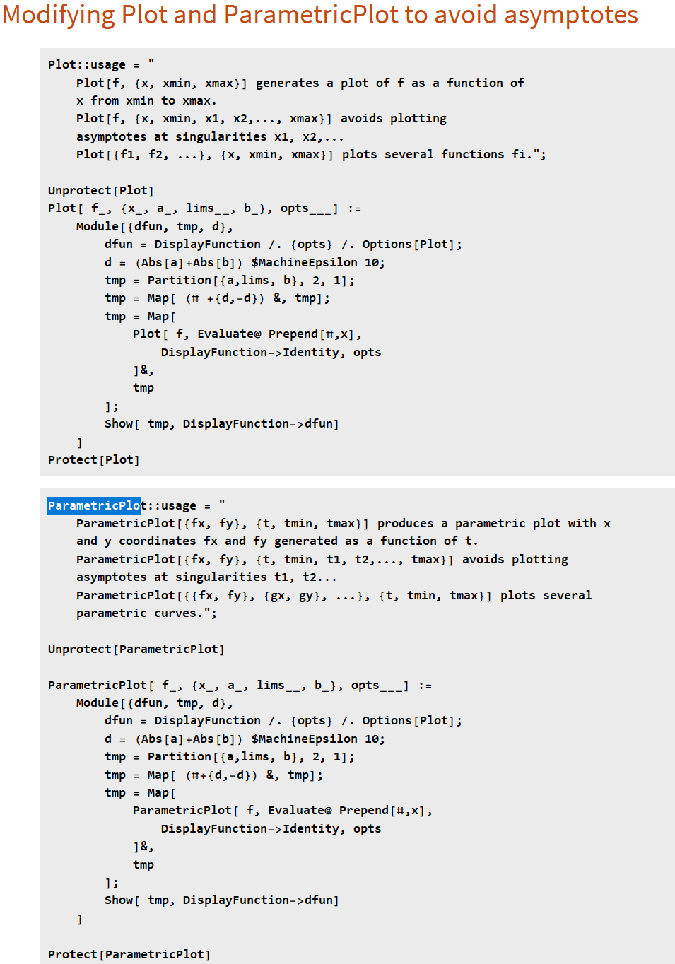
Plot::usage = "
	Plot[f, {x, xmin, xmax}] generates a plot of f as a function of
	x from xmin to xmax.
	Plot[f, {x, xmin, x1, x2,..., xmax}] avoids plotting
	asymptotes at singularities x1, x2,...
	Plot[{f1, f2, ...}, {x, xmin, xmax}] plots several functions fi.";

Unprotect[Plot]
Plot[ f_, {x_, a_, lims__, b_}, opts___] :=
	Module[{dfun, tmp, d},
		dfun = DisplayFunction /. {opts} /. Options[Plot];
		d = (Abs[a]+Abs[b]) $MachineEpsilon 10;
		tmp = Partition[{a,lims, b}, 2, 1];
		tmp = Map[ (# +{d,-d}) &, tmp];
		tmp = Map[
			Plot[ f, Evaluate@ Prepend[#,x],
				DisplayFunction->Identity, opts
			]&,
			tmp
		];
		Show[ tmp, DisplayFunction->dfun]
	]
Protect[Plot]
ParametricPlot::usage = "
	ParametricPlot[{fx, fy}, {t, tmin, tmax}] produces a parametric plot with x
	and y coordinates fx and fy generated as a function of t.
	ParametricPlot[{fx, fy}, {t, tmin, t1, t2,..., tmax}] avoids plotting
	asymptotes at singularities t1, t2...
	ParametricPlot[{{fx, fy}, {gx, gy}, ...}, {t, tmin, tmax}] plots several
	parametric curves.";

Unprotect[ParametricPlot]

ParametricPlot[ f_, {x_, a_, lims__, b_}, opts___] :=
	Module[{dfun, tmp, d},
		dfun = DisplayFunction /. {opts} /. Options[Plot];
		d = (Abs[a]+Abs[b]) $MachineEpsilon 10;
		tmp = Partition[{a,lims, b}, 2, 1];
		tmp = Map[ (#+{d,-d}) &, tmp];
		tmp = Map[
			ParametricPlot[ f, Evaluate@ Prepend[#,x],
				DisplayFunction->Identity, opts
			]&,
			tmp
		];
		Show[ tmp, DisplayFunction->dfun]
	]

Protect[ParametricPlot]