Wolfram: Plot and Visualization

Math Visualization and Graphics Functions

There are two major types of builtin plotting functions:

• Plot math functions. e.g. plot sine, equation, vector valued function, complex function, parametric formula for 2D or 3D, etc.
• Plot data (usually list of numbers), such as pie chart, bar chart, statistics, histogram, stock chart, or a surface by a bunch of points, etc.

Find Math Plot Functions

?*Plot*

list all functions containing the name “Plot”. (return value is wrapped in InformationDataGrid so it is clickable in notebook to goto doc.)

full syntax is

Information["*Plot*"]

FunctionVisualization

Names["*Plot*"]

Return a list of names.

?*Plot*

(* InformationDataGrid[{System` -> {AbsArgPlot, AnatomyPlot3D, ArrayPlot, ArrayPlot3D, AudioPlot, BioSequencePlot, BodePlot, ChromaticityPlot, ChromaticityPlot3D, CommunityGraphPlot, ComplexArrayPlot, ComplexContourPlot, ComplexListPlot, ComplexPlot, ComplexPlot3D, ComplexRegionPlot, ComplexStreamPlot, ComplexVectorPlot, ContourPlot, ContourPlot3D, CumulativeFeatureImpactPlot, DateListLogPlot, DateListPlot, DateListStepPlot, DensityPlot, DensityPlot3D, DiscretePlot, DiscretePlot3D, FeatureImpactPlot, FeatureSpacePlot, FeatureSpacePlot3D, FeatureValueDependencyPlot, FeatureValueImpactPlot, GeoContourPlot, GeoDensityPlot, GeoGraphPlot, GeoGraphValuePlot, GeoListPlot, GeoRegionValuePlot, GeoStreamPlot, GeoVectorPlot, GraphPlot, GraphPlot3D, ImageVectorscopePlot, ImageWaveformPlot, JuliaSetPlot, LayeredGraphPlot, LayeredGraphPlot3D, LineIntegralConvolutionPlot, ListContourPlot, ListContourPlot3D, ListCurvePathPlot, ListDensityPlot, ListDensityPlot3D, ListLineIntegralConvolutionPlot, ListLinePlot, ListLinePlot3D, ListLogLinearPlot, ListLogLogPlot, ListLogPlot, ListPlot, ListPlot3D, ListPointPlot3D, ListPolarPlot, ListSliceContourPlot3D, ListSliceDensityPlot3D, ListSliceVectorPlot3D, ListStepPlot, ListStreamDensityPlot, ListStreamPlot, ListStreamPlot3D, ListSurfacePlot3D, ListVectorDensityPlot, ListVectorDisplacementPlot, ListVectorDisplacementPlot3D, ListVectorPlot, ListVectorPlot3D, LogLinearPlot, LogLogPlot, LogPlot, MandelbrotSetPlot, MatrixPlot, MaxPlotPoints, MoleculePlot, MoleculePlot3D, NicholsPlot, NumberLinePlot, NyquistPlot, PairwiseListPlot, PairwiseProbabilityPlot, PairwiseQuantilePlot, ParallelAxisPlot, ParametricPlot, ParametricPlot3D, Plot, Plot3D, Plot3Matrix, PlotDivision, PlotHighlighting, PlotJoined, PlotLabel, PlotLabels, PlotLayout, PlotLegends, PlotMarkers, PlotPoints, PlotRange, PlotRangeClipping, PlotRangeClipPlanesStyle, PlotRangePadding, PlotRegion, PlotStyle, PlotTheme, PointValuePlot, PolarPlot, ProbabilityPlot, ProbabilityScalePlot, QuantilePlot, RadialAxisPlot, RegionPlot, RegionPlot3D, ReImPlot, ReliefPlot, RevolutionPlot3D, RootLocusPlot, RulePlot, SingularValuePlot, SliceContourPlot3D, SliceDensityPlot3D, SliceVectorPlot3D, SphericalPlot3D, StackedDateListPlot, StackedListPlot, StreamDensityPlot, StreamPlot, StreamPlot3D, SystemModelPlot, SystemModelUncertaintyPlot, TernaryListPlot, TernaryPlotCorners, TimelinePlot, TreePlot, VectorDensityPlot, VectorDisplacementPlot, VectorDisplacementPlot3D, VectorPlot, VectorPlot3D, WaveletImagePlot, WaveletListPlot, WaveletMatrixPlot, $PlotTheme}}, False] *)

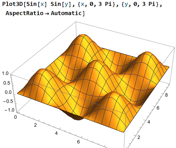
Plot3D[Sin[x] Sin[y], {x,0, 3 Pi }, {y,0, 3 Pi }, AspectRatio -> Automatic]

Functions for Data Visualization

e.g. BarChart, PieChart, Histogram, BoxWhiskerChart, etc.

• DataVisualization

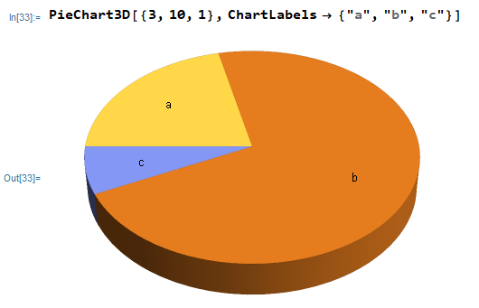
PieChart3D[{3, 10, 1}, ChartLabels -> {"a", "b", "c"}]

Find Options of Functions

Plot functions have many optional parameters.

Type Options[ FunctionName ] to get a list of options for the function.

Options[ Plot ]

(* {AlignmentPoint -> Center, AspectRatio -> GoldenRatio^(-1), Axes -> True, AxesLabel -> None, AxesOrigin -> Automatic, AxesStyle -> {}, Background -> None, BaselinePosition -> Automatic, BaseStyle -> {}, ClippingStyle -> None, ColorFunction -> Automatic, ColorFunctionScaling -> True, ColorOutput -> Automatic, ContentSelectable -> Automatic, CoordinatesToolOptions -> Automatic, DisplayFunction :> $DisplayFunction, Epilog -> {}, Evaluated -> Automatic, EvaluationMonitor -> None, Exclusions -> Automatic, ExclusionsStyle -> None, Filling -> None, FillingStyle -> Automatic, FormatType :> TraditionalForm, Frame -> False, FrameLabel -> None, FrameStyle -> {}, FrameTicks -> Automatic, FrameTicksStyle -> {}, GridLines -> None, GridLinesStyle -> {}, ImageMargins -> 0., ImagePadding -> All, ImageSize -> Automatic, ImageSizeRaw -> Automatic, LabelingSize -> Automatic, LabelStyle -> {}, MaxRecursion -> Automatic, Mesh -> None, MeshFunctions -> {#1 & }, MeshShading -> None, MeshStyle -> Automatic, Method -> Automatic, PerformanceGoal :> $PerformanceGoal, PlotHighlighting -> Automatic, PlotLabel -> None, PlotLabels -> None, PlotLayout -> Automatic, PlotLegends -> None, PlotPoints -> Automatic, PlotRange -> {Full, Automatic}, PlotRangeClipping -> True, PlotRangePadding -> Automatic, PlotRegion -> Automatic, PlotStyle -> Automatic, PlotTheme :> $PlotTheme, PreserveImageOptions -> Automatic, Prolog -> {}, RegionFunction -> (True & ), RotateLabel -> True, ScalingFunctions -> None, TargetUnits -> Automatic, Ticks -> Automatic, TicksStyle -> {}, WorkingPrecision -> MachinePrecision} *)

Type ?Name to get the documentation for the option name.

?Axes

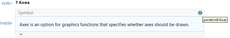
Click the info icon to goto the full documentation.