Astroid

History

The cycloidal curves, including the astroid, were discovered by Roemer (1674) in his search for the best form for gear teeth. Double generation was first noticed by Daniel Bernoulli in 1725.

From E H Lockwood A book of Curves (1961):

The astroid seems to have acquired its present name only in 1838, in a book published in Vienna; it went, even after that time, under various other names, such as cubocycloid, paracycle, four-cusp-curve, and so on. The equation x^(2/3) + y^(2/3) == a^(2/3) can, however, be found in Leibniz's correspondence as early as 1715.

Description

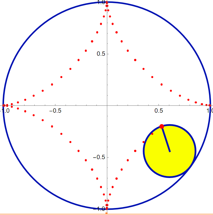
Astroid is a special case of hypotrochoid. (See: Curve Family Index). Astroid is defined as the trace of a point on a circle rolling inside a fixed circle of radius 1, the rolling circle has radius 1/4.

astroid 4 roll circle JN7wM

Clear[hypotrochoidAnimate]

hypotrochoidAnimate::usage = "
hypotrochoidAnimate[{a,b,h}]
generates a list of graphics that trace out a hypotrochoid by rolling a circle inside another.

a is the radius of the fixed circle.
b is the radius of the rolling circle.
a > b.
h is the distance from the tracing point to the center of the rolling circle.

hypotrochoidAnimate[{a,b,h}, {tMin, tMax}]
start at tMin, stop at tMax.
{tMin, tMax} control the number of rotations.

hypotrochoidAnimate[{a,b,h}, {tMin, tMax, tStep}]
using tStep.

hypotrochoidAnimate[ {1, 1/4, 1/4}, {0, 2 Pi, 2 Pi/10} ]

If not specified, an internal algorithm will figure out the number of rotations so that the curve is closed.

tStep control the number of frames indirectly.

0 <= tMin <= tMax < Infinity.

Options:

NumberOfFrames-> Automatic
LastFrameOnly -> False

example:

ListAnimate @ hypotrochoidAnimate[ {1, 1/4, 1/4} ]

ListAnimate @ hypotrochoidAnimate[ {1, 1/4, 1/4}, {0, Pi, 0.2 } ]

hypotrochoidAnimate[ {1, 1/4, 1/4}, LastFrameOnly -> True ]

hypotrochoidAnimate[ {1, 1/4, 1/4}, {0, Pi}, LastFrameOnly -> True ]

ListAnimate @ hypotrochoidAnimate[ {1, 3/4, 3/4}, NumberOfFrames -> 100 ]

hypotrochoidAnimate[ {1, 2/5, 1}, LastFrameOnly -> True, NumberOfFrames -> Automatic]

hypotrochoidAnimate[ {1, 1/3, 1/3}, LastFrameOnly -> True, NumberOfFrames -> 120]

Created: 2026-03-01
Version: 2026-03-06
";

Options[hypotrochoidAnimate] =
  Join[{NumberOfFrames -> Automatic, LastFrameOnly -> False},
   Options[Graphics]];

hypotrochoidAnimate[{a_, b_, h_}, tRange_List : Automatic,
  opts : OptionsPattern[]] :=
 Block[{nOfFrames, tMin, tMax, tStep, xmargin, tRangeList,
   tracingPointF, pointListGP, staticGP, movingGP,
   lastFrameGP},
(* 2026-03-06 todo. set the number of frames such that the tracing point traveled after tStep is constant like 0.3*)
  nOfFrames =
   If[OptionValue @ NumberOfFrames === Automatic,
    Min[400, ((Numerator @ Rationalize[b/a, 0])  (15*4))],
    OptionValue @ NumberOfFrames];
  {tMin, tMax, tStep} =
   Which[tRange === Automatic, {0,
     N @ Numerator @ Rationalize[N @ b/a, 0]  2  Pi,
     N @ (tMax - tMin)/(nOfFrames - 1)}, Length @ tRange === 3, N @ tRange,
    True, N @ {First @ tRange, Last @ tRange, (tMax - tMin)/(nOfFrames - 1)}];
  xmargin = (a + Max[0, h - b])  1.05;
  tRangeList = N @ Range[tMin, tMax, tStep];
  tracingPointF =
   Compile[{x}, {(a - b)  Cos[x] +
      h  Cos[-(a - b)/b  x], (a - b)  Sin[x] + h  Sin[-(a - b)/b  x]}];
  pointListGP = Map[Function[Point @ tracingPointF @ #], tRangeList];
  staticGP = {Hue[.65, 1, .7], Thickness[.007], Circle[{0, 0}, a]};
  movingGP =
   Function[
    Block[{xcenter},
xcenter = N @ (a - b) {Cos[tMin + (# - 1) tStep], Sin[tMin + (# - 1) tStep]} ;
{
{Hue[.17], Disk[xcenter, b]}
,
{Hue[.65, 1, .7], Thickness[.008], Circle[xcenter, b], Line[{xcenter, pointListGP[[#, 1]]}]} ,
{Hue[0], PointSize[.02], pointListGP[[#]]}
}]];
  Table[Graphics[{staticGP, movingGP @ nn, Hue[0],
     Take[pointListGP, nn]}, FilterRules[{opts}, Options[Graphics]],
    AspectRatio -> Automatic, Axes -> True,
    PlotRange -> ({{-1, 1}, {-1, 1}}  xmargin)], {nn,
    Evaluate @ If[OptionValue @ LastFrameOnly, Length @ tRangeList, 1],
    Length @ tRangeList}]]

(*s------------------------------*)

ListAnimate @ hypotrochoidAnimate[{1, 1/4, 1/4}]

ListAnimate @ hypotrochoidAnimate[{1, 1/4, 1/4}, {0, Pi, 0.2}]

hypotrochoidAnimate[{1, 1/4, 1/4}, LastFrameOnly -> True]

hypotrochoidAnimate[{1, 1/4, 1/4}, {0, Pi}, LastFrameOnly -> True]

ListAnimate @ hypotrochoidAnimate[{1, 3/4, 3/4}, NumberOfFrames -> 100]

hypotrochoidAnimate[{1, 2/5, 1}, LastFrameOnly -> True,
 NumberOfFrames -> Automatic]

hypotrochoidAnimate[{1, 1/3, 1/3}, LastFrameOnly -> True,
 NumberOfFrames -> 120]

Or, the the rolling circle radius is 3/4. This is known as double generation.

astroid double gen KgS8M Astroid as Hypotrochoid, double generation.

GeoGebra: Astroid Roll .

The two sizes of rolling circles that generate the astroid can be synchronized by a linkage. (this means: the 2 roulette methods trace the curve with the same speed and has a geometric relation)
Let A be the center of the fixed circle.
Let D be the center of the smaller rolling circle.
Let F be a fixed point on this circle (the tracing point).
Let G be a point translated from A by the vector DF.
G is the center of the large rolling circle, with the same tracing point at F.
ADFG is a parallelogram with sides having constant lengths.

Formula

The following formulas describe a astroid centered on the origin, and the length from center to one cusp is a, where a is a scaling factor.

(*xahnote: prove astroid eq from parametric: (x^2 +y^2 -1)^3 + 27 * x^2 * y^2 == 0 is equivalent to x^(2/3) + y^(2/3) == 1. And, in general, what are the exhaustive list of operations are allow on f[x]==0 to generate the same curve? where f is not necessarily polynomial.*)

Parametric: {Cos[t]^3, Sin[t]^3}, 0 < t ≤ 2 Pi.

Cartesian: (x^2 +y^2 -1)^3 + 27 * x^2 * y^2 == 0. Expanded: -1 + 3*x^2 - 3*x^4 + x^6 + 3*y^2 + 21*x^2*y^2 + 3*x^4*y^2 - 3*y^4 + 3*x^2*y^4 + y^6 == 0.

This equation is centered on origin and a cusp at {1,0}. Replace x by x/a and y by y/a and multiply both sides by a^6 and we obtain the classic equation given with scaling factor a as: (x^2 + y^2 - a^2)^3 + 27*a^2*x^2*y^2 == 0.

another equivalent equation is: x^(2/3) + y^(2/3) == 1.

astroid_eq_proof.nb

Curve Construction

The astroid is rich in properties that one can construct the curve, its tangent, and center of osculating circle, and device other mechanical ways to generate the curve.

Let there be a circle c centered on B passing K. We will construct a astroid centered on O with one cusp at K. Let O be the origin, and K be the point {1,0}. Let L be a point on c. Drop a line from L perpendicular to x-axis, let M be their intersection. Similarly drop a line from L perpendicular to y-axis, call the intersection N. Let P be a point on MN such that LP and MN are perpendicular. Now, P is a point on the astroid, and MN is its tangent, LP is its normal. Let D be the intersection of LP and c. Let D' be the reflection of D thru MN. Now, D' is the center of osculating circle at P.

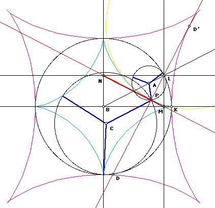
astroid construction — GeoGebra: Astroid Construction

prove this contruction of curve point, and tangent. It can be done by analytic geometry. By matching the equation of the construction with the parametric formula based on rolling circle. The construction of the curvature center can also be done similarly by matching formula. However, at least for the curve point case, it would be interseting and perhaps not too difficult to find a geometric proof. Partial done: astroid_const2.ggb

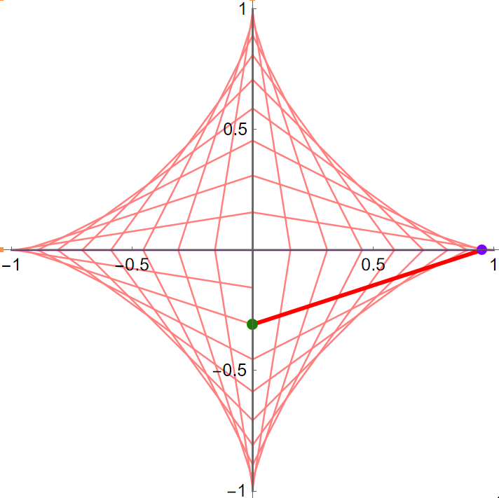
Trammel of Archimedes

Define the axes of the astroid to be the two perpendicular lines passing its cusps. Property: The length of tangent cut by the axes is constant.

A mechanical devise where a fixed bar with endings sliding on two perpendicular tracks is called the Trammel of Archimedes. The envelope of the moving bar is then the astroid. A fixed point on the bar will trace out a ellipse. (see left figure)

astroid trammal CJwVS

(* 2026-02-26 *)

Clear[astroidTrammelAnimate]

astroidTrammelAnimate::usage = "astroidTrammelAnimate[] generates an animation of astroid by Trammel of Archimedes.
return a list of Graphics.

astroidTrammelAnimate[{tMin, tMax, tStep}]
generation animation from tMin to tMax by tStep.
by default, they are {0, 2 Pi, 2 Pi / 40}
";

astroidTrammelAnimate[] = astroidTrammelAnimate[{0, 2 Pi, 2 Pi / 40}];

astroidTrammelAnimate[{tmin_, tmax_}] = astroidTrammelAnimate[{tmin, tmax, (tmax - tmin) / 40}];

astroidTrammelAnimate[{tmin_, tmax_ , tstep_}] :=

Block[{tRangeList, lineListGP,staticGP, movingGPFn},

 tRangeList = Range[tmin, tmax, tstep];
 lineListGP = (Line[{{Cos@#,0},{0,Sin@#}}]&) /@ tRangeList;

 staticGP = {Hue[.75], Line[{{-1,0},{1,0}}],Hue[.3,1,.5],Line[{{0,-1},{0,1}}]};

 movingGPFn = Function @
  { Red, Thickness[.008], Line @ {{Cos@#,0},{0,Sin@#}},
   Purple, PointSize[.02], Point @ {Cos@#,0},
    Hue[.3,1,.5], Point @ {0,Sin@#}
  };

Table[
Graphics[ {Hue[0,.5,1], Take[ lineListGP,t], staticGP, movingGPFn@ tRangeList[[t]] },
AspectRatio->Automatic, Axes->True,
Ticks->{{-1,-.5,.5,1},{-1,-.5,.5,1}},
PlotRange->{{-1.05,1.05},{-1.05,1.05}}
],
   {t, Length@tRangeList}
  ]
]

(* s------------------------------ *)

ListAnimate @ astroidTrammelAnimate[]

GeoGebra: Astroid Trammel .

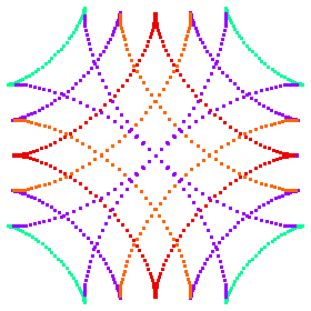
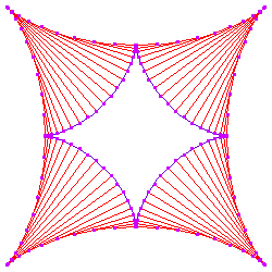
Envelope of Ellipses

Astroid is the envelope of co-axial ellipses whose sum of major and minor axes is contsant.

astroid by ellipse 7SFN8 — Envelope of Ellipses

ParametricPlot[
Table[ {xi Cos@t, (1 -xi) Sin@t}, {xi, 0, 1, 1/5. } ]
,
{ t, 0, 2 Pi}]

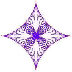
Evolute of Astroid

The evolute of a astroid is another astroid. (all epi/hypocycloids' evolute is equal to themselves)

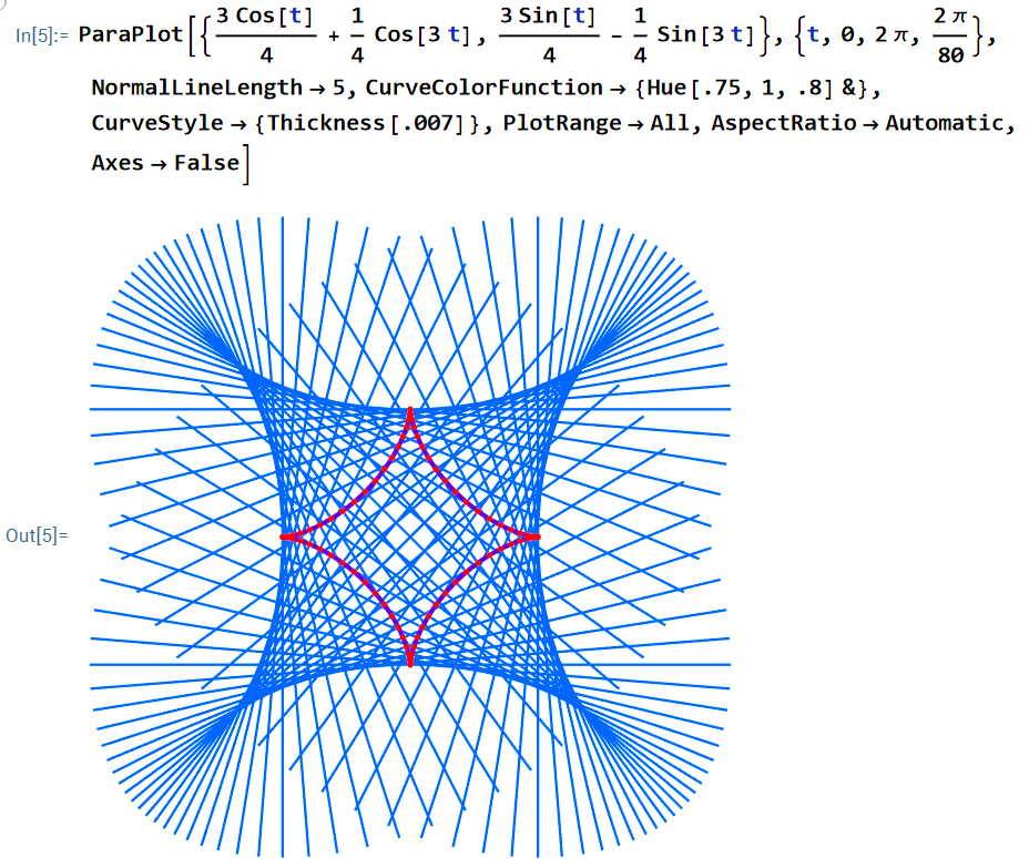
astroidEvolute points on the curve are connected to their center of osculating circles.

astroid normals tQtcr the evolute is drawn as the envelope of normals.

ParaPlot[
{(3 Cos[t])/4 + 1/4 Cos[3 t], (3 Sin[t])/4 - 1/4 Sin[3 t]},
{t, 0, 2 Pi, (2 Pi)/80},
 NormalLineLength -> 5, CurveColorFunction -> {Hue[.75, 1, .8] &},
 CurveStyle -> {Thickness[.007]}, PlotRange -> All,
 AspectRatio -> Automatic, Axes -> False]

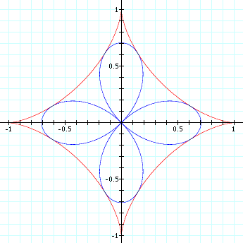
Pedal, Radial, and Rose

The pedal of a astroid with respect to its center is 4 petalled rose, called a quadrifolium. Astroid's radial is also quadrifolium. (all epi/hypocycloid's pedal and radial are equal, and they are roses.)

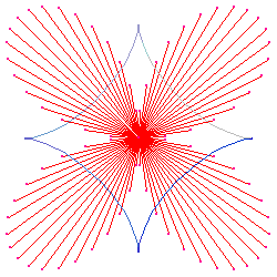
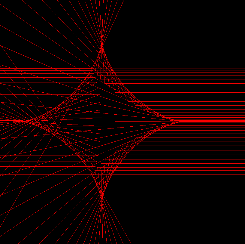
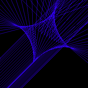
Deltoid and Astroid

Astroid is the catacaustic of deltoid with parallel rays in any direction.

deltoid caustic astroid — Moving Light Source

Orthoptic

The orthoptic with respect to its center is r^2 == (1/2)*Cos[2*θ]^2. (Robert Yates) Recall that a orthoptic of a curve is the locus of all points where the curve's tangents meet at right angles. prove astroid's orthoptic